Interpreting the GUI
Our BAMS article on SHARPpy provides an overview of the various insets and information included in the SHARPpy sounding window. Included within the paper is a list of references to journal articles which describe the relevance of each aspect of the SHARPpy sounding window to research in atmospheric science and the scientific forecasting process. This documentation repeats some of the information included in the BAMS article and describes the various parts of the SHARPpy GUI.
Additional resources for interpreting the GUI include the SPC Sounding Analysis Help and Explanation of SPC Severe Weather Parameters webpages. The first site describes the SHARP GUI, which is the basis for the SHARPpy GUI. The second can be used to help interpret some of the various convection indices shown in the SHARPpy GUI. Not all features shown on these two sites are shown in the SHARPpy GUI.
Skew-T
Various sounding variables are displayed in the Skew-T, which is a central panel of the GUI:
Solid red – temperature profile
Solid green – dewpoint profile
Dashed red – virtual temperature profile.
Solid cyan – wetbulb temperature profile
Dashed white – parcel trace (e.g., MU, SFC, ML) (the parcel trace of the parcel highlighted in yellow in the Thermodynamic Inset.)
Dashed purple – downdraft parcel trace (parcel origin height is at minimum 100-mb mean layer equivalent potenial temperature).
Winds barbs are plotted in knots (unless switched to m/s in the preferences) and are interpolated to 50-mb intervals for visibility purposes.
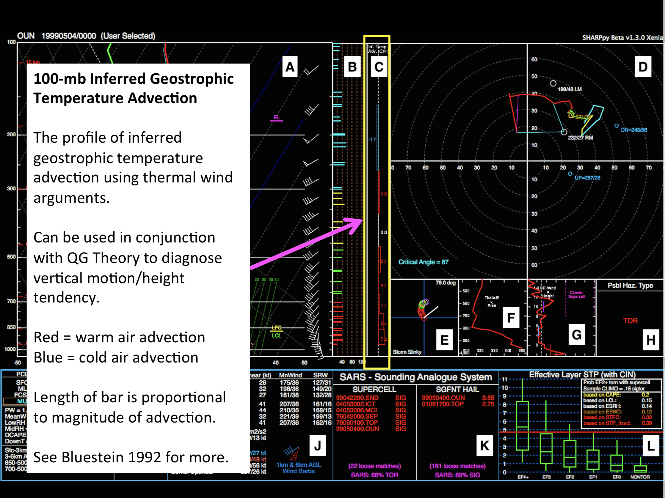
If a vertical velocity profile (omega) is found (e.g., sounding is from a model), it is plotted on the left. Blue bars indicate sinking motion, red bars rising motion. Dashed purple lines indicate the bounds of synopic scale vertical motion. Units of the vertical velocity are in microbars/second.
Note
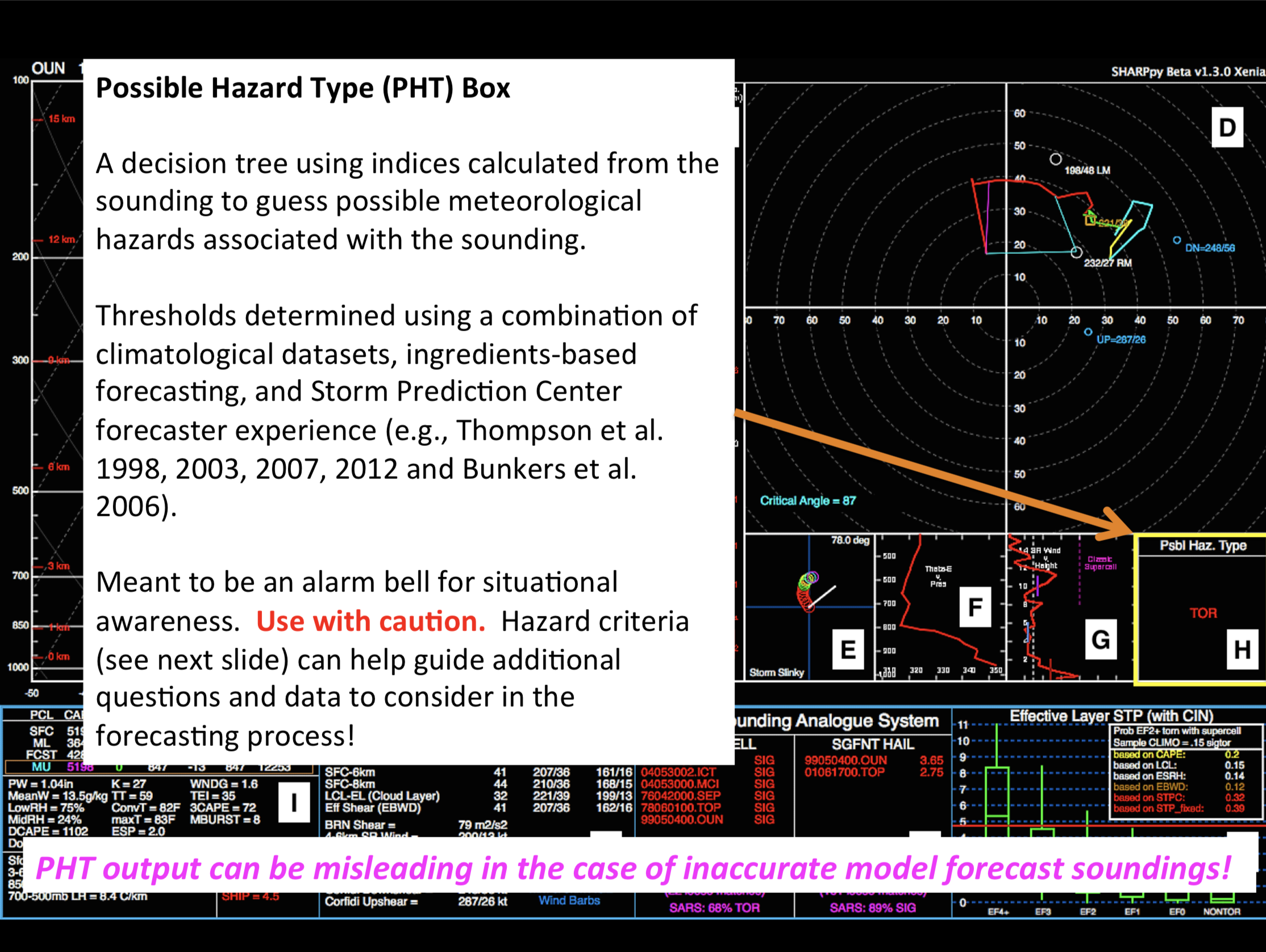
When analyzing model forecast soundings, the omega profile can be used to determine whether or not models are “convectively contaminated”. This phrase means that the sounding being viewed is under the influence of convection and therefore is not representitive of the large-scale environment surrounding the storm. When omega values become much larger than synoptic scale vertical motion values, users should take care to when interpreting the data.
Parcel LCL, LFC, and EL are denoted on the right-hand side in green, yellow and purple, respectively. Levels where the environmental temperature are 0, -20, and -30 C are labeled in dark blue. The cyan and purple I-bars indicate the effective inflow layer and the layer with the maximum lapse rate between 2-6 km AGL. Information about the effective inflow layer may be found in Thompson et al. 2007.
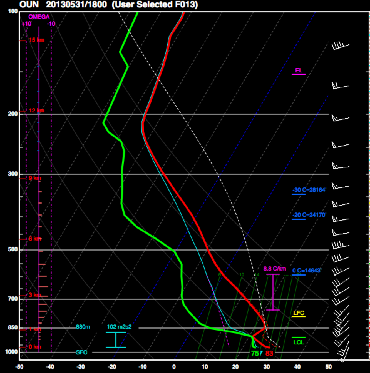
An example of the Skew-T inset showing a model forecast sounding for May 31, 2013 at 18 UTC. The 2-6 km max lapse rate layer clearly denotes the elevated mixed layer, while the omega profile indicates that rising motion is occuring within the lowest 6 km of the sounding in the forecast.
If the Winter inset is selected, SHARPpy will label the the dendritic growth zone (DGZ), the wet-bulb zero (WBZ), and the freezing level (FRZ) on the Skew-T diagram. If the Fire inset is selected, the convective boundary layer top will be denoted on the Skew-T.
Wind Speed Profile
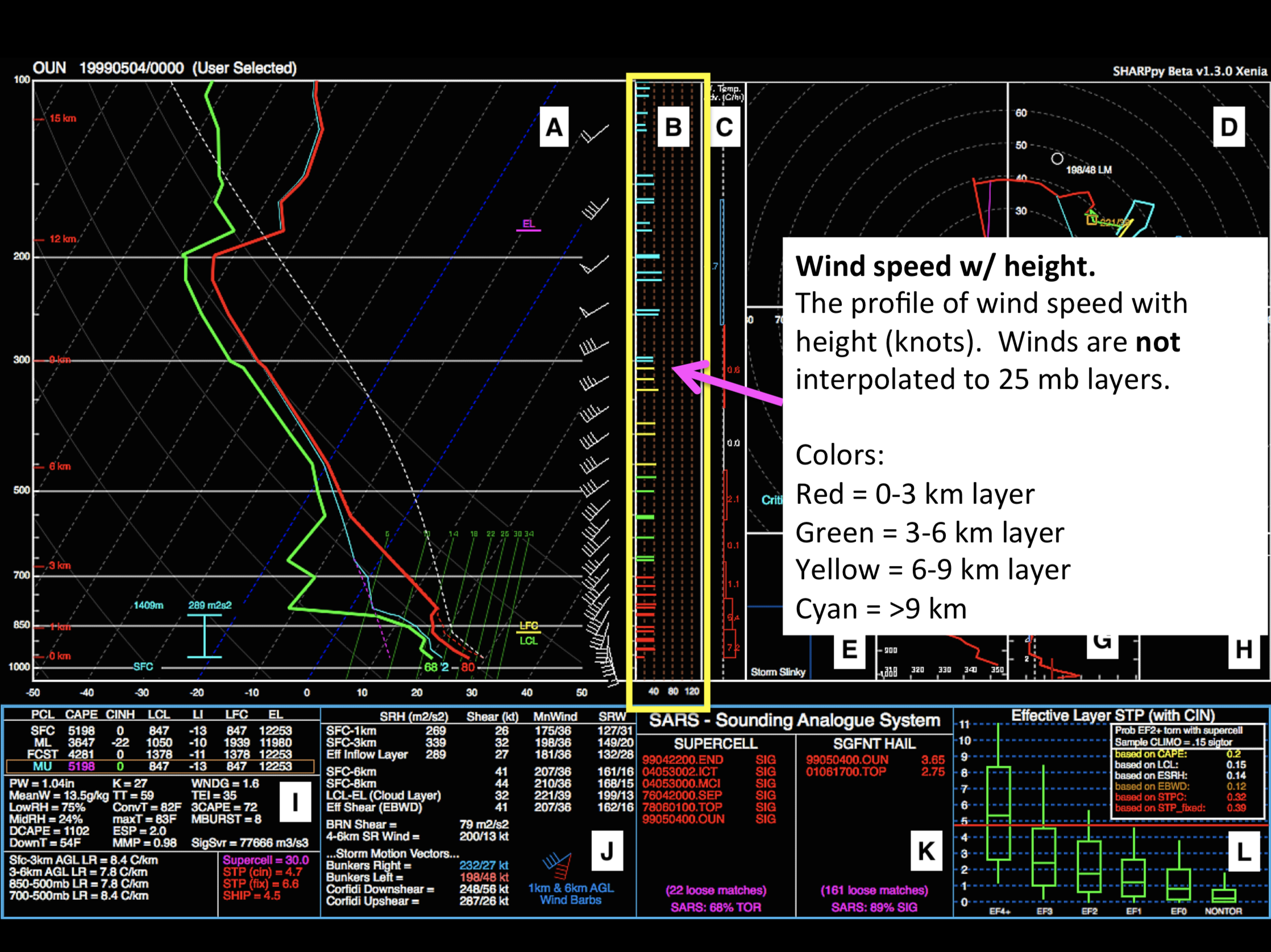
The tick marks for this plot are every 20 knots (should knots be the default unit selected in the preferences).
Inferred Temperature Advection Profile
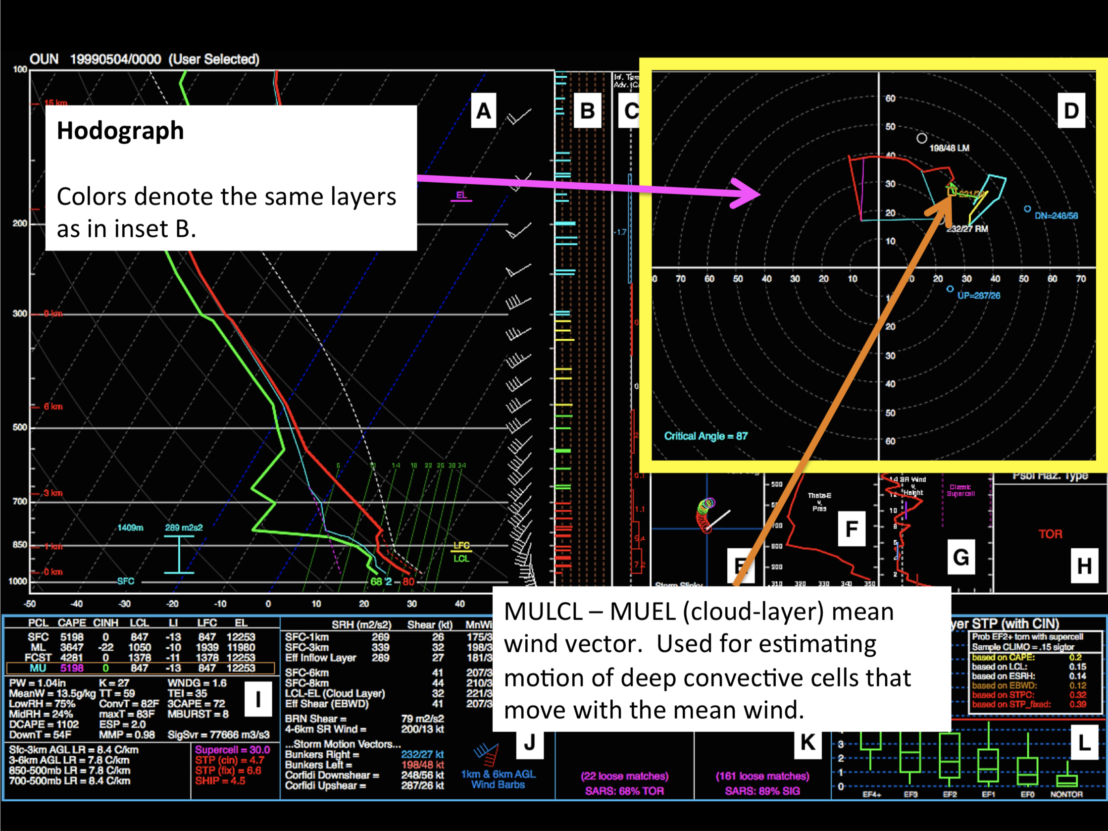
Hodograph
Although the hodograph plotted follows the traditional convention used throughout meteorology, the hodograph shown here is broken up into layers by color. In addition, several vectors are also plotted from different SHARPpy algorithms.
Bunkers Storm Motion Vectors
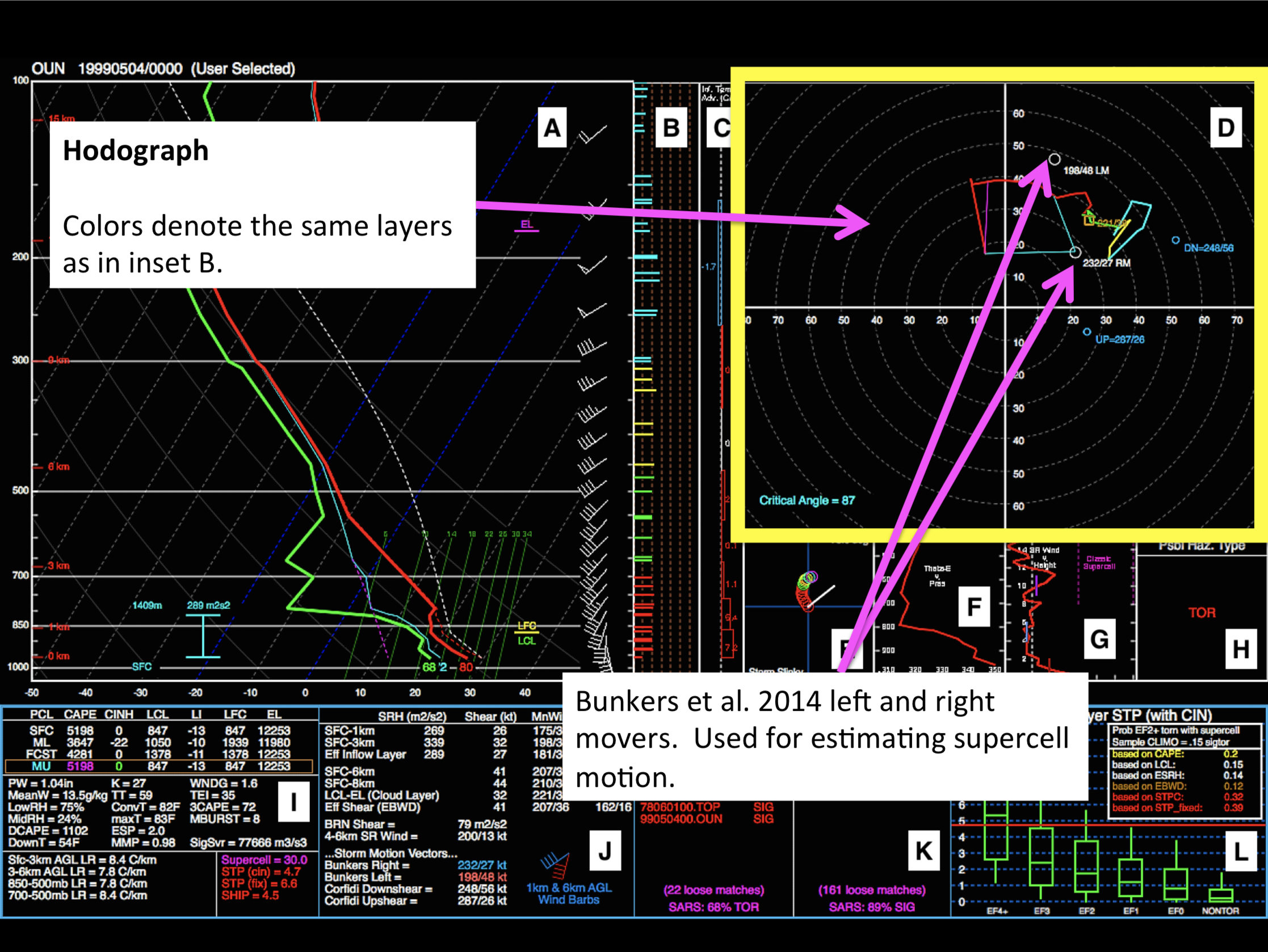
The storm motion vectors here are computed using the updated Bunkers et al. 2014 algorithm, which takes into account the effective inflow layer.
Corfidi Vectors
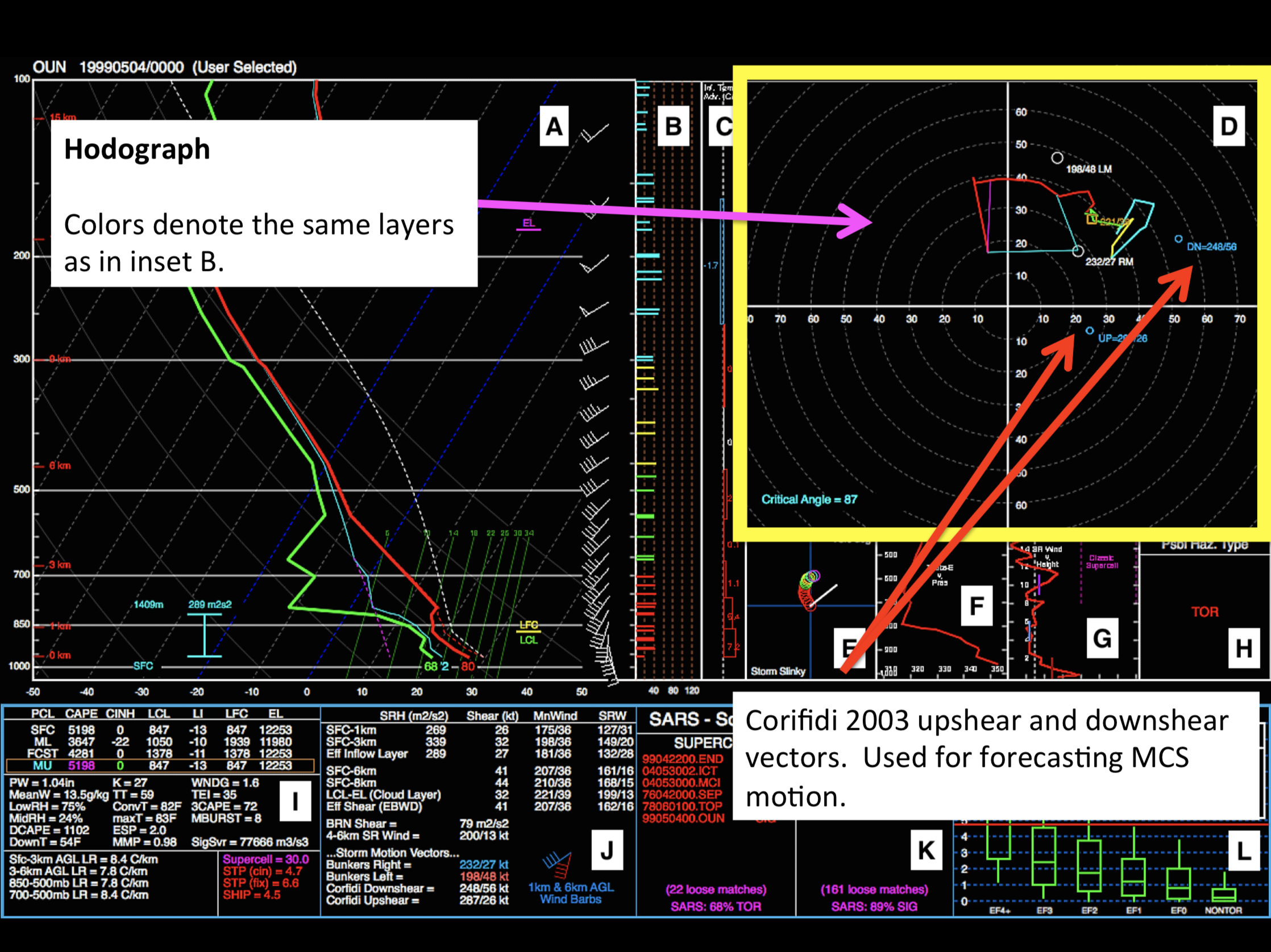
The Corfidi vectors may be used to estimate mesoscale convective system (MCS) motion. See Corfidi 2003 for more information about how these are calculated.
LCL-EL Mean Wind
Critical Angle
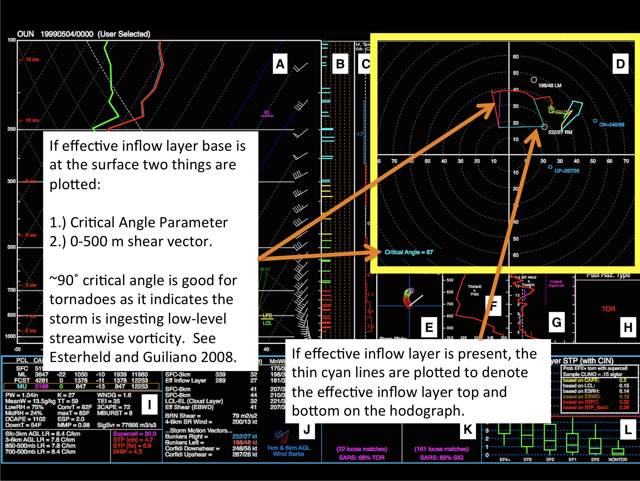
See Esterheld and Guiliano 2008 for more information on the use of critical angle in forecasting.

Theta-E w/ Pressure
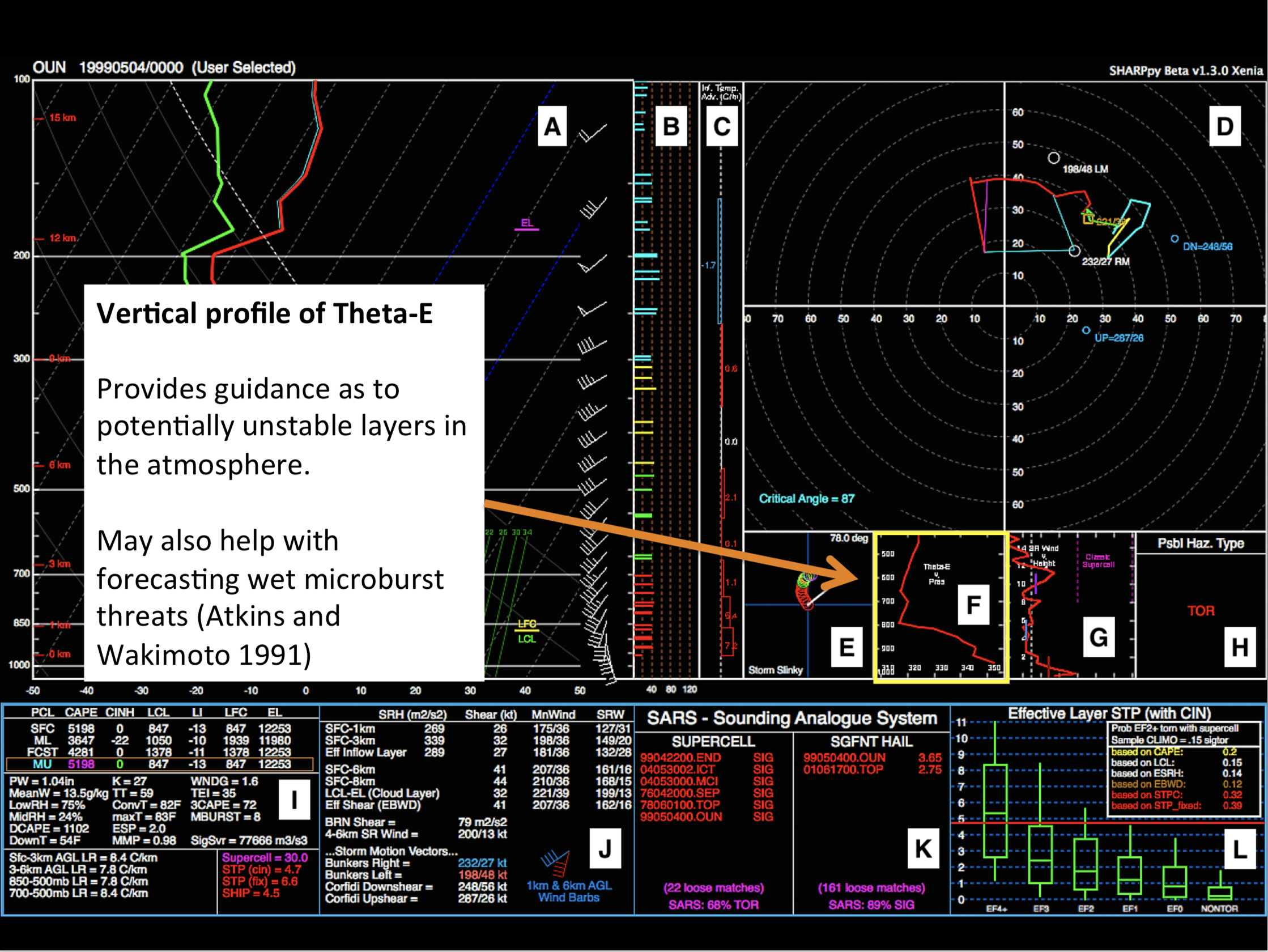
See Atkins and Wakimoto 1991 for more information on what to look for in this inset when forecasting wet microbursts.
Storm-Relative Winds w/ Height
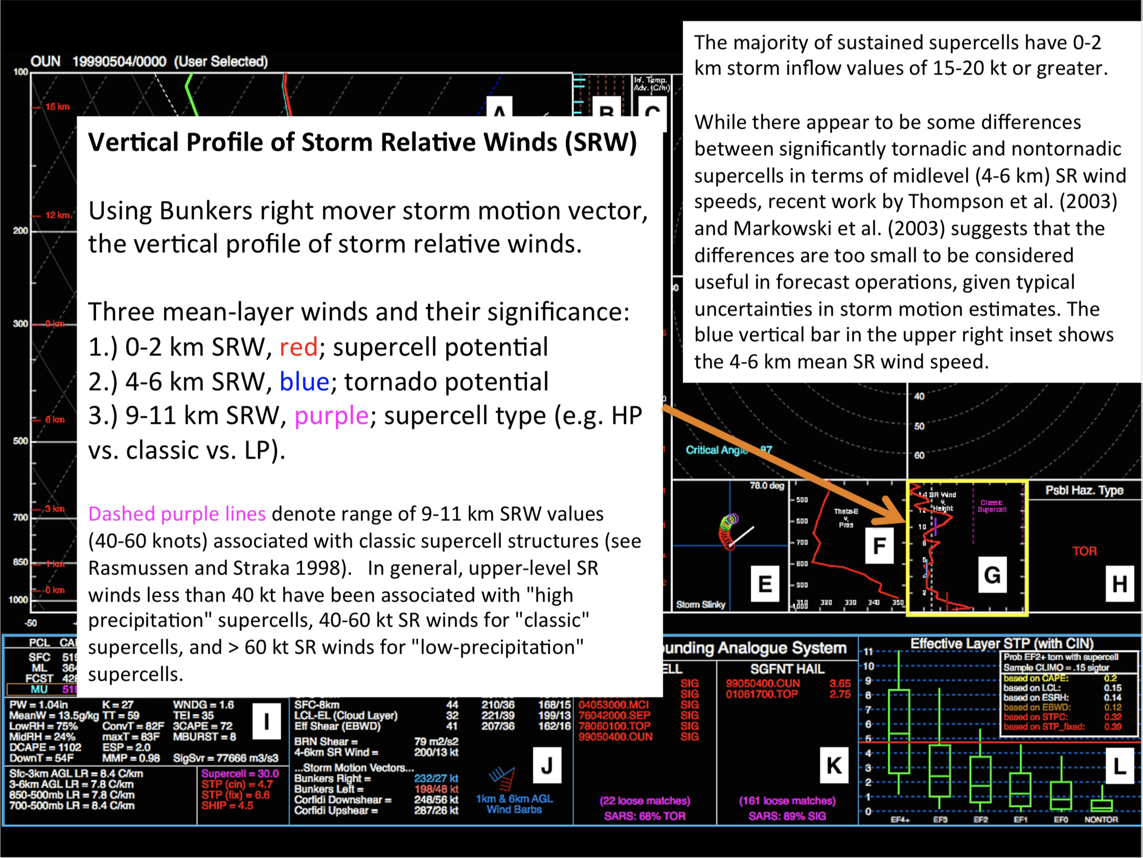
See Rasmussen and Straka 1998 for more information on how the anvil-level storm relative winds may be used to predict supercell morphology. See Thompson et al. 2003 for information on using the 4-6 km storm-relative winds to predict tornado environments.