Scripting¶

This tutorial is meant to teach the user how to directly interact with the SHARPpy libraries using the Python interpreter. This tutorial will cover reading in files into the the Profile object, plotting the data using Matplotlib, and computing various indices from the data. It is also a reference to the different functions and variables SHARPpy has available to the user.

3 Steps to Scripting¶

For those wishing to run SHARPpy routines using Python scripts, you often will need to perform 3 steps before you can begin running routines. These three steps read in the data, load in the SHARPpy modules, and convert the data into SHARPpy Profile objects.

Step 1: Load in the modules.¶

All of the SHARPpy routines (parcel lifting, composite indices, etc.) reside within the SHARPTAB module.

SHARPTAB contains 6 modules: params, winds, thermo, utils, interp, fire, constants, watch_type

Each module has different functions:

interp - interpolates different variables (temperature, dewpoint, wind, etc.) to a specified pressure
winds - functions used to compute different wind-related variables (shear, helicity, mean winds, storm relative vectors)
thermo - temperature unit conversions, theta-e, theta, wetbulb, lifting functions
utils - wind speed unit conversions, wind speed and direction to u and v conversions, QC
params - computation of different parameters, indices, etc. from the Profile object
fire - fire weather indices

Below is the code to load in these modules:

import sharppy
import sharppy.sharptab.profile as profile
import sharppy.sharptab.interp as interp
import sharppy.sharptab.winds as winds
import sharppy.sharptab.utils as utils
import sharppy.sharptab.params as params
import sharppy.sharptab.thermo as thermo

To learn more about the functions available in SHARPTAB, access the API here: Module Index

Step 2: Read in the data.¶

For this example, the Pilger, NE tornado proximity sounding from 19 UTC within the tutorial/ directory is an example of the SPC sounding file format that can be read in by the GUI. Here we’ll read it in manually.

If you want to read in your own data using this function, write a script to mimic the data format shown in the 14061619.OAX file found in this directory. Missing values must be -9999. We’ll have to also load in Matplotlib for this example (which comes default with Anaconda) to plot some of the data.

import matplotlib as pyplot.plt
spc_file = open('14061619.OAX', 'r').read()

Step 3: Make a Profile object.¶

Before running any analysis routines on the data, we have to create a Profile object first. A Profile object describes the vertical thermodynamic and kinematic profiles and is the key object that all SHARPpy routines need to run. Any data source can be passed into a Profile object (i.e. radiosonde, RASS, satellite sounding retrievals, etc.) as long as it has these profiles:

temperature (C)
dewpoint (C)
height (meters above mean sea level)
pressure (millibars)
wind speed (kts)
wind direction (degrees)

or (optional) - zonal wind component U (kts) - meridional wind component V (kts)

For example, after reading in the data in the example above, a Profile object can be created. Since this file uses the value -9999 to indicate missing values, we need to tell SHARPpy to ignore these values in its calculations by including the missing field to be -9999. In addition, we tell SHARPpy we want to create a default BasicProfile object. Telling SHARPpy to create a “convective” profile object instead of a “default” profile object will generate a Profile object with all of the indices computed in the SHARPpy GUI. If you are only wanting to compute a few indices, you probably don’t want to do that.

import numpy as np
from StringIO import StringIO

def parseSPC(spc_file):
    """
        This function will read a SPC-style formatted observed sounding file,
        similar to that of the 14061619.OAX file included in the SHARPpy distribution.

        It will return the pressure, height, temperature, dewpoint, wind direction and wind speed data
        from that file.
    """
    ## read in the file
    data = np.array([l.strip() for l in spc_file.split('\n')])

    ## necessary index points
    title_idx = np.where( data == '%TITLE%')[0][0]
    start_idx = np.where( data == '%RAW%' )[0] + 1
    finish_idx = np.where( data == '%END%')[0]

    ## create the plot title
    data_header = data[title_idx + 1].split()
    location = data_header[0]
    time = data_header[1][:11]

    ## put it all together for StringIO
    full_data = '\n'.join(data[start_idx : finish_idx][:])
    sound_data = StringIO( full_data )

    ## read the data into arrays
    p, h, T, Td, wdir, wspd = np.genfromtxt( sound_data, delimiter=',', comments="%", unpack=True )

    return p, h, T, Td, wdir, wspd

pres, hght, tmpc, dwpc, wdir, wspd = parseSPC(spc_file)

prof = profile.create_profile(profile='default', pres=pres, hght=hght, tmpc=tmpc, \
                                    dwpc=dwpc, wspd=wspd, wdir=wdir, missing=-9999, strictQC=True)

Important

In SHARPpy, Profile objects have quality control checks built into them to alert the user to bad data and in order to prevent the program from crashing on computational routines. For example, upon construction of the Profile object, the SHARPpy will check for unrealistic values (i.e. dewpoint or temperature below absolute zero, negative wind speeds) and incorrect ordering of the height and pressure arrays. Height arrays must be increasing with array index, and pressure arrays must be decreasing with array index. Repeat values are not allowed. If you encounter this issue, you can either manually edit the data to remove the offending data values or you can avoid these checks by setting the “strictQC” flag to False when constructing an object.

Tip

Because Python is an interpreted language, it can be quite slow for certain processes. When working with soundings in SHARPpy, we recommend the profiles contain a maximum of 200-500 points. High resolution radiosonde profiles (i.e. 1 second profiles) contain thousands of points and some of the SHARPpy functions that involve lifting parcels (i.e. parcelx) may take a long time to run. To filter your data to make it easier for SHARPpy to work with, you can use a sounding filter such as the one found here:

https://github.com/tsupinie/SoundingFilter

Viewing the Profiles¶

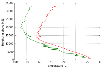
Data can be plotted using Matplotlib by accessing the attributes of the Profile object. Below is an example of Python code plotting the temperature and dewpoint profiles with height:

import matplotlib.pyplot as plt
plt.plot(prof.tmpc, prof.hght, 'r-')
plt.plot(prof.dwpc, prof.hght, 'g-')
#plt.barbs(40*np.ones(len(prof.hght)), prof.hght, prof.u, prof.v)
plt.xlabel("Temperature [C]")
plt.ylabel("Height [m above MSL]")
plt.grid()
plt.show()

SHARPpy Profile objects keep track of the height grid the profile lies on. Within the profile object, the height grid is assumed to be in meters above mean sea level.

In the example data provided, the profile can be converted to and from AGL from MSL:

msl_hght = prof.hght[prof.sfc] # Grab the surface height value
print("SURFACE HEIGHT (m MSL):",msl_hght)
agl_hght = interp.to_agl(prof, msl_hght) # Converts to AGL
print("SURFACE HEIGHT (m AGL):", agl_hght)
msl_hght = interp.to_msl(prof, agl_hght) # Converts to MSL
print("SURFACE HEIGHT (m MSL):",msl_hght)

SURFACE HEIGHT (m MSL): 350.0
SURFACE HEIGHT (m AGL): 0.0
SURFACE HEIGHT (m MSL): 350.0

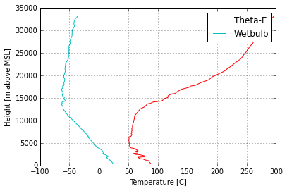
By default, Profile objects also create derived profiles such as Theta-E and Wet-Bulb when they are constructed. These profiles are accessible to the user too.

plt.plot(thermo.ktoc(prof.thetae), prof.hght, 'r-', label='Theta-E')
plt.plot(prof.wetbulb, prof.hght, 'c-', label='Wetbulb')
plt.xlabel("Temperature [C]")
plt.ylabel("Height [m above MSL]")
plt.legend()
plt.grid()
plt.show()

Lifting parcels¶

In SHARPpy, parcels are lifted via the params.parcelx() routine. The parcelx() routine takes in the arguments of a Profile object and a flag to indicate what type of parcel you would like to be lifted. Additional arguments can allow for custom/user defined parcels to be passed to the parcelx() routine, however most users will likely be using only the Most-Unstable, Surface, 100 mb Mean Layer, and Forecast parcels.

The parcelx() routine by default utilizes the virtual temperature correction to compute variables such as CAPE and CIN. If the dewpoint profile contains missing data, parcelx() will disregard using the virtual temperature correction.

sfcpcl = params.parcelx( prof, flag=1 ) # Surface Parcel
fcstpcl = params.parcelx( prof, flag=2 ) # Forecast Parcel
mupcl = params.parcelx( prof, flag=3 ) # Most-Unstable Parcel
mlpcl = params.parcelx( prof, flag=4 ) # 100 mb Mean Layer Parcel

Once your parcel attributes are computed by params.parcelx(), you can extract information about the parcel such as CAPE, CIN, LFC height, LCL height, EL height, etc. We will do this for the Most Unstable parcel mupcl.

print("Most-Unstable CAPE:", mupcl.bplus) # J/kg
print("Most-Unstable CIN:", mupcl.bminus) # J/kg
print("Most-Unstable LCL:", mupcl.lclhght) # meters AGL
print("Most-Unstable LFC:", mupcl.lfchght) # meters AGL
print("Most-Unstable EL:", mupcl.elhght) # meters AGL
print("Most-Unstable LI:", mupcl.li5) # C

This code outputs the following text:

Most-Unstable CAPE: 5769.22545311
Most-Unstable CIN: -0.644692447001
Most-Unstable LCL: 512.718558828
Most-Unstable LFC: 612.53643485
Most-Unstable EL: 13882.5821154
Most-Unstable LI: -13.8145334959

The six indices listed above are not the only ones calculated by parcelx(). Other indices can be calculated and accessed too:

Here is a list of the attributes and their units contained in each parcel object (pcl):

pcl.pres - Parcel beginning pressure (mb)
pcl.tmpc - Parcel beginning temperature (C)
pcl.dwpc - Parcel beginning dewpoint (C)
pcl.ptrace - Parcel trace pressure (mb)
pcl.ttrace - Parcel trace temperature (C)
pcl.blayer - Pressure of the bottom of the layer the parcel is lifted (mb)
pcl.tlayer - Pressure of the top of the layer the parcel is lifted (mb)
pcl.lclpres - Parcel LCL (lifted condensation level) pressure (mb)
pcl.lclhght - Parcel LCL height (m AGL)
pcl.lfcpres - Parcel LFC (level of free convection) pressure (mb)
pcl.lfchght - Parcel LFC height (m AGL)
pcl.elpres - Parcel EL (equilibrium level) pressure (mb)
pcl.elhght - Parcel EL height (m AGL)
pcl.mplpres - Maximum Parcel Level (mb)
pcl.mplhght - Maximum Parcel Level (m AGL)
pcl.bplus - Parcel CAPE (J/kg)
pcl.bminus - Parcel CIN (J/kg)
pcl.bfzl - Parcel CAPE up to freezing level (J/kg)
pcl.b3km - Parcel CAPE up to 3 km (J/kg)
pcl.b6km - Parcel CAPE up to 6 km (J/kg)
pcl.p0c - Pressure value at 0 C  (mb)
pcl.pm10c - Pressure value at -10 C (mb)
pcl.pm20c - Pressure value at -20 C (mb)
pcl.pm30c - Pressure value at -30 C (mb)
pcl.hght0c - Height value at 0 C (m AGL)
pcl.hghtm10c - Height value at -10 C (m AGL)
pcl.hghtm20c - Height value at -20 C (m AGL)
pcl.hghtm30c - Height value at -30 C (m AGL)
pcl.wm10c - Wet bulb velocity at -10 C
pcl.wm20c - Wet bulb velocity at -20 C
pcl.wm30c - Wet bulb at -30 C
pcl.li5 = - Lifted Index at 500 mb (C)
pcl.li3 = - Lifted Index at 300 mb (C)
pcl.brnshear - Bulk Richardson Number Shear
pcl.brnu - Bulk Richardson Number U (kts)
pcl.brnv - Bulk Richardson Number V (kts)
pcl.brn - Bulk Richardson Number (unitless)
pcl.limax - Maximum Lifted Index (C)
pcl.limaxpres - Pressure at Maximum Lifted Index (mb)
pcl.cap - Cap Strength (C)
pcl.cappres - Cap strength pressure (mb)
pcl.bmin - Buoyancy minimum in profile (C)
pcl.bminpres - Buoyancy minimum pressure (mb)

Calculating kinematic indicies¶

SHARPpy also allows the user to compute kinematic variables such as shear, mean-winds, and storm relative helicity. SHARPpy will also compute storm motion vectors based off of the work by Stephen Corfidi and Matthew Bunkers. Below is some example code to compute the following:

0-3 km Pressure-Weighted Mean Wind
0-6 km Shear (kts)
Bunker’s Storm Motion (right-mover) (Bunkers et al. 2014 version)
Bunker’s Storm Motion (left-mover) (Bunkers et al. 2014 version)
0-3 km Storm Relative Helicity

# Find the pressure values that correspond to the surface, 1 km, 3 km and 6 km levels.
sfc = prof.pres[prof.sfc]
p3km = interp.pres(prof, interp.to_msl(prof, 3000.))
p6km = interp.pres(prof, interp.to_msl(prof, 6000.))
p1km = interp.pres(prof, interp.to_msl(prof, 1000.))

# Calculate the 0-3 km pressure-weighted mean wind
mean_3km = winds.mean_wind(prof, pbot=sfc, ptop=p3km)
print("0-3 km Pressure-Weighted Mean Wind (kt):", utils.comp2vec(mean_3km[0], mean_3km[1])[1])

# Calculate the 0-1, 0-3, and 0-6 km wind shear
sfc_6km_shear = winds.wind_shear(prof, pbot=sfc, ptop=p6km)
sfc_3km_shear = winds.wind_shear(prof, pbot=sfc, ptop=p3km)
sfc_1km_shear = winds.wind_shear(prof, pbot=sfc, ptop=p1km)
print("0-6 km Shear (kt):", utils.comp2vec(sfc_6km_shear[0], sfc_6km_shear[1])[1])

# Calculate the Bunkers Storm Motion Left and Right mover vectors (these are returned in u,v space
# so let's transform them into wind speed and direction space.)
srwind = params.bunkers_storm_motion(prof)
print("Bunker's Storm Motion (right-mover) [deg,kts]:", utils.comp2vec(srwind[0], srwind[1]))
print("Bunker's Storm Motion (left-mover) [deg,kts]:", utils.comp2vec(srwind[2], srwind[3]))

# Calculate the storm-relative helicity using the right-movers
srh3km = winds.helicity(prof, 0, 3000., stu = srwind[0], stv = srwind[1])
srh1km = winds.helicity(prof, 0, 1000., stu = srwind[0], stv = srwind[1])
print("0-3 km Storm Relative Helicity [m2/s2]:",srh3km[0])

This code outputs the following text:

0-3 km Pressure-Weighted Mean Wind (kt): 41.1397595603
0-6 km Shear (kt): 55.9608928026
Bunker's Storm Motion (right-mover) [deg,kts]: (masked_array(data = 225.652934838,
             mask = False,
       fill_value = -9999.0)
, 27.240749559186799)
Bunker's Storm Motion (left-mover) [deg,kts]: (masked_array(data = 204.774711769,
             mask = False,
       fill_value = -9999.0)
, 52.946150880598658)
0-3 km Storm Relative Helicity [m2/s2]: 584.016767705

Calculating other indices¶

The effective inflow layer is occasionally used to derive other variables that may be used to explain a storm’s behavior. Here are a few examples of how to compute variables that require the effective inflow layer in order to calculate them:

# Let's calculate the effective inflow layer and print out the heights of the top
# and bottom of the layer.  We'll have to convert it from m MSL to m AGL.
eff_inflow = params.effective_inflow_layer(prof)
ebot_hght = interp.to_agl(prof, interp.hght(prof, eff_inflow[0]))
etop_hght = interp.to_agl(prof, interp.hght(prof, eff_inflow[1]))
print("Effective Inflow Layer Bottom Height (m AGL):", ebot_hght)
print("Effective Inflow Layer Top Height (m AGL):", etop_hght)

# Like before, we can calculate the storm-relative helicity, but let's do it for the effective inflow layer.
effective_srh = winds.helicity(prof, ebot_hght, etop_hght, stu = srwind[0], stv = srwind[1])
print("Effective Inflow Layer SRH (m2/s2):", effective_srh[0])

# We can also calculate the Effective Bulk Wind Difference using the wind shear calculation and the inflow layer.
ebwd = winds.wind_shear(prof, pbot=eff_inflow[0], ptop=eff_inflow[1])
ebwspd = utils.mag( ebwd[0], ebwd[1] )
print("Effective Bulk Wind Difference:", ebwspd)

# Composite indices (e.g. STP, SCP, SHIP) can be calculated after determining the effective inflow layer.
scp = params.scp(mupcl.bplus, effective_srh[0], ebwspd)
stp_cin = params.stp_cin(mlpcl.bplus, effective_srh[0], ebwspd, mlpcl.lclhght, mlpcl.bminus)
stp_fixed = params.stp_fixed(sfcpcl.bplus, sfcpcl.lclhght, srh1km[0], utils.comp2vec(sfc_6km_shear[0], sfc_6km_shear[1])[1])
ship = params.ship(prof)
print("Supercell Composite Parameter:", scp)
print("Significant Tornado Parameter (w/CIN):", stp_cin)
print("Significant Tornado Parameter (fixed):", stp_fixed)
print("Significant Hail Parameter:", ship)

This code then will output this text:

Effective Inflow Layer Bottom Height (m AGL): 0.0
Effective Inflow Layer Top Height (m AGL): 2117.98
Effective Inflow Layer SRH (m2/s2): 527.913472562
Effective Bulk Wind Difference: 43.3474336034
Supercell Composite Parameter: 60.9130368589
Significant Tornado Parameter (w/CIN): 13.8733427141
Significant Tornado Parameter (fixed): 13.6576402964

Plotting a Skew-T using Matplotlib¶

Now, let’s try to plot the data on a Skew-T. You may want to do this if you’re looking to create a plot for use in a publication.

First, we need to tell Matplotlib (the Python plotting package) that we’d like a Skew-T style plot. This can be done by using the code found at: http://matplotlib.org/examples/api/skewt.html

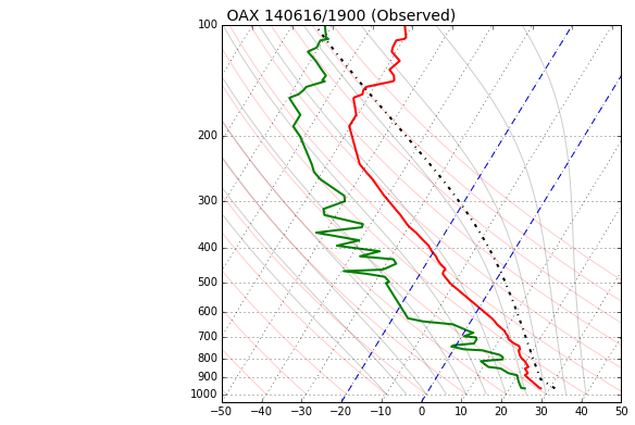
Now that Matplotlib knows about the Skew-T style plot, let’s plot the OAX sounding data on a Skew-T and show the Most-Unstable parcel trace. Let’s also include dry adiabats and moist adiabats for the user.

# Create a new figure. The dimensions here give a good aspect ratio
import sharppy.plot.skew as skew
fig = plt.figure(figsize=(6.5875, 6.2125))
ax = fig.add_subplot(111, projection='skewx')
ax.grid(True)

# Select the Most-Unstable parcel (this can be changed)
pcl = mupcl

# Let's set the y-axis bounds of the plot.
pmax = 1000
pmin = 10
dp = -10
presvals = np.arange(int(pmax), int(pmin)+dp, dp)

# plot the moist-adiabats at surface temperatures -10 C to 45 C at 5 degree intervals.
for t in np.arange(-10,45,5):
    tw = []
    for p in presvals:
        tw.append(thermo.wetlift(1000., t, p))
    # Plot the moist-adiabat with a black line that is faded a bit.
    ax.semilogy(tw, presvals, 'k-', alpha=.2)

# A function to calculate the dry adiabats
def thetas(theta, presvals):
    return ((theta + thermo.ZEROCNK) / (np.power((1000. / presvals),thermo.ROCP))) - thermo.ZEROCNK

# plot the dry adiabats
for t in np.arange(-50,110,10):
    ax.semilogy(thetas(t, presvals), presvals, 'r-', alpha=.2)

# plot the title.
plt.title(' OAX 140616/1900 (Observed)', fontsize=14, loc='left')

# Plot the data using normal plotting functions, in this case using
# log scaling in Y, as dicatated by the typical meteorological plot
ax.semilogy(prof.tmpc, prof.pres, 'r', lw=2)
ax.semilogy(prof.dwpc, prof.pres, 'g', lw=2)

# Plot the parcel trace.
ax.semilogy(pcl.ttrace, pcl.ptrace, 'k-.', lw=2)

# Denote the 0 to -20 C area on the Skew-T.
l = ax.axvline(0, color='b', linestyle='--')
l = ax.axvline(-20, color='b', linestyle='--')

# Set the log-scale formatting and label the y-axis tick marks.
ax.yaxis.set_major_formatter(plt.ScalarFormatter())
ax.set_yticks(np.linspace(100,1000,10))
ax.set_ylim(1050,100)

# Label the x-axis tick marks.
ax.xaxis.set_major_locator(plt.MultipleLocator(10))
ax.set_xlim(-50,50)

# Show the plot to the user.
# plt.savefig('skewt.png', bbox_inches='tight') # saves the plot to the disk.
plt.show()